An introduction to the phyloregion package

Barnabas H. Daru, Piyal Karunarathne & Klaus Schliep

January 27, 2024

1. Installation

phyloregion is available from the Comprehensive R Archive Network, so you can use the following line of code to install and run it:

install.packages("phyloregion")

Alternatively, you can install the development version of phyloregion hosted on GitHub. To do this, you will need to install the devtools package. In R, type:

if (!requireNamespace("remotes", quietly = TRUE)) 
    install.packages("remotes") 
remotes::install_github("darunabas/phyloregion")

When installed, load the package in R:

library(phyloregion)

2. Overview and general workflow of phyloregion

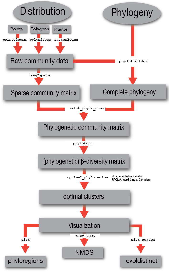
The workflow of the phyloregion package demonstrates steps from preparation of different types of data to visualizing the results of biogeographical regionalization, together with tips on selecting the optimal method for achieving the best output, depending on the types of data used and research questions.

Figure 1. Simplified workflow for analysis of biogeographical regionalization using phyloregion. Distribution data is converted to a sparse community matrix. When paired with phylogenetic data, phylobuilder creates a subtree with largest overlap from a species list, thereby ensuring complete representation of missing data; phylocommunity matrix to visualization of results.

3. Input data

Phylogenies

In R, phylogenetic relationships among species / taxa are often represented as a phylo object implemented in the ape package(Paradis and Schliep 2018). Phylogenies (often in the Newick or Nexus formats) can be imported into R with the read.tree or read.nexus functions of the ape package(Paradis and Schliep 2018).

library(ape)
library(Matrix)
library(terra)

## terra 1.7.55

## 
## Attaching package: 'terra'

## The following objects are masked from 'package:ape':
## 
##     rotate, trans, zoom

data(africa)
sparse_comm <- africa$comm

tree <- africa$phylo
tree <- keep.tip(tree, intersect(tree$tip.label, colnames(sparse_comm)))
par(mar=c(2,2,2,2))
plot(tree, show.tip.label=FALSE)

Figure 2. Phylogenetic tree of the woody plants of southern Africa inferred from DNA barcodes using a maximum likelihood approach and transforming branch lengths to millions of years ago by enforcing a relaxed molecular clock and multiple calibrations (Barnabas H. Daru, Bank, and Davies 2015).

Distribution data input

The phyloregion package has functions for manipulating three kinds of distribution data: point records, vector polygons and raster layers. An overview can be easily obtained with the functions points2comm, polys2comm and rast2comm for point records, polygons, or raster layers, respectively. Depending on the data source, all three functions ultimately provide convenient interfaces to convert the distribution data to a community matrix at varying spatial grains and extents for downstream analyses.

We will play around with these functions in turn.

Function points2comm

Here, we will generate random points in geographic space, similar to occurrence data obtained from museum records, GBIF, iDigBio, or CIESIN which typically have columns of geographic coordinates for each observation.

s <- vect(system.file("ex/nigeria.json", package="phyloregion"))

set.seed(1)
m <- as.data.frame(spatSample(s, 1000, method = "random"),
                   geom = "XY")[-1]
names(m) <- c("lon", "lat")
species <- paste0("sp", sample(1:100))
m$taxon <- sample(species, size = nrow(m), replace = TRUE)

pt <- points2comm(dat = m, res = 0.5, lon = "lon", lat = "lat",
            species = "taxon") # This generates a list of two objects
head(pt[[1]][1:5, 1:5])

## 5 x 5 sparse Matrix of class "dgCMatrix"
##      sp1 sp10 sp100 sp11 sp12
## v100   .    .     .    .    .
## v101   .    1     .    .    .
## v102   .    .     .    .    .
## v103   .    .     .    .    .
## v105   .    .     .    .    .

Function polys2comm

This function converts polygons to a community matrix at varying spatial grains and extents for downstream analyses. Polygons can be derived from the IUCN Redlist spatial database (https: //www.iucnredlist.org/resources/spatial-data-download), published monographs or field guides validated by taxonomic experts. To illustrate this function, we will use the function random_species to generate random polygons for five random species over the landscape of Nigeria as follows:

s <- vect(system.file("ex/nigeria.json", package="phyloregion"))
sp <- random_species(100, species=5, pol=s)
pol <- polys2comm(dat = sp)
head(pol[[1]][1:5, 1:5])

## 5 x 5 sparse Matrix of class "dgCMatrix"
##       species1 species2 species3 species4 species5
## v10          .        .        .        1        .
## v100         .        .        .        1        1
## v1000        .        .        .        1        1
## v1001        .        .        .        1        1
## v1002        .        .        .        1        1

Function rast2comm

This third function, converts raster layers (often derived from species distribution modeling, such as aquamaps(Kaschner et al. 2008)) to a community matrix.

fdir <- system.file("NGAplants", package="phyloregion")
files <- file.path(fdir, dir(fdir))
ras <- rast2comm(files) 
head(ras[[1]][1:5, 1:5])

## 5 x 5 sparse Matrix of class "dgCMatrix"
##      Chytranthus_gilletii Commelina_ramulosa Cymbopogon_caesius
## v100                    .                  .                  .
## v101                    .                  .                  .
## v102                    .                  .                  .
## v103                    .                  .                  .
## v104                    .                  .                  .
##      Dalechampia_ipomoeifolia Grewia_barombiensis
## v100                        1                   .
## v101                        1                   .
## v102                        1                   .
## v103                        1                   .
## v104                        1                   .

The object ras above also returns two objects: a community data frame and a vector of grid cells with the numbers of species per cell and can be plotted as a heatmap using plot function as follows:

s <- vect(system.file("ex/SR_Naija.json", package="phyloregion"))
par(mar=rep(0,4))
plot(s, "SR", border=NA, type = "continuous", 
     col = hcl.colors(20, palette = "Blue-Red 3", rev=FALSE))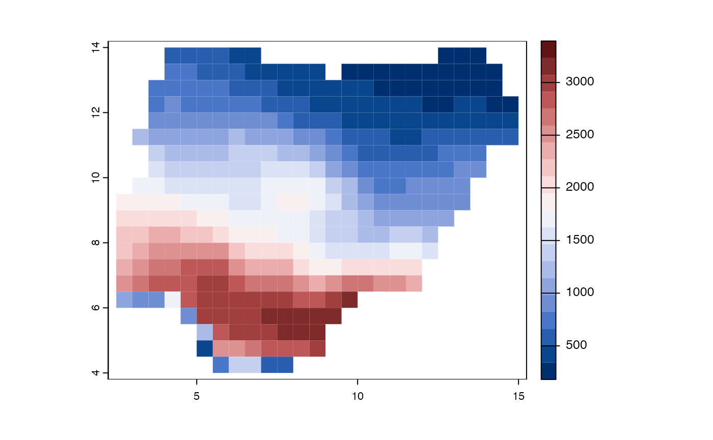

Figure 3. Species richness of plants in Nigeria across equal area grid cells. This is to demonstrate how the function plot works.

Community data

Community data are commonly stored in a matrix with the sites as rows and species / operational taxonomic units (OTUs) as columns. The elements of the matrix are numeric values indicating the abundance/observations or presence/absence (0/1) of OTUs in different sites. In practice, such a matrix can contain many zero values because species are known to generally have unimodal distributions along environmental gradients (Ter Braak and Prentice 2004), and storing and analyzing every single element of that matrix can be computationally challenging and expensive.

phyloregion differs from other R packages (e.g. vegan (Oksanen et al. 2019), picante (Kembel et al. 2010) or betapart(Baselga and Orme 2012)) in that the data are not stored in a (dense) matrix or data.frame but as a sparse matrix making use of the infrastructure provided by the Matrix package (Bates and Maechler 2019). A sparse matrix is a matrix with a high proportion of zero entries(Duff 1977), of which only the non-zero entries are stored and used for downstream analysis.

A sparse matrix representation has two advantages. First the community matrix can be stored in a much memory efficient manner, allowing analysis of larger datasets. Second, for very large datasets spanning thousands of taxa and spatial scales, computations with a sparse matrix are often much faster.
The phyloregion package contains functions to conveniently change between data formats.

library(Matrix) 
data(africa)
sparse_comm <- africa$comm
dense_comm <- as.matrix(sparse_comm) 
object.size(dense_comm)

## 4216952 bytes

object.size(sparse_comm)

## 885952 bytes

Here, the data set in the dense matrix representation consumes roughly five times more memory than the sparse representation.

4. Analysis

Alpha diversity

We demonstrate the utility of phyloregion in mapping standard conservation metrics of species richness, weighted endemism (weighted_endemism) and threat (map_traits) as well as fast computations of phylodiversity measures such as phylogenetic diversity (PD), phylogenetic endemism (phylo_endemism), and evolutionary distinctiveness and global endangerment (EDGE). The major advantage of these functions compared to available tools is the ability to utilize sparse matrix that speeds up the analyses without exhausting computer memories, making it ideal for handling any data from small local scales to large regional and global scales.

Function weighted_endemism

Weighted endemism is species richness inversely weighted by species ranges(Crisp et al. 2001),(Laffan and Crisp 2003),(Barnabas H. Daru et al. 2020).

library(terra)
data(africa)
p <- vect(system.file("ex/sa.json", package = "phyloregion"))
Endm <- weighted_endemism(africa$comm)
m <- merge(p, data.frame(grids=names(Endm), WE=Endm), by="grids")
m <- m[!is.na(m$WE),]

par(mar=rep(0,4))
plot(m, "WE", col = hcl.colors(20, "Blue-Red 3"), 
     type="continuous", border = NA)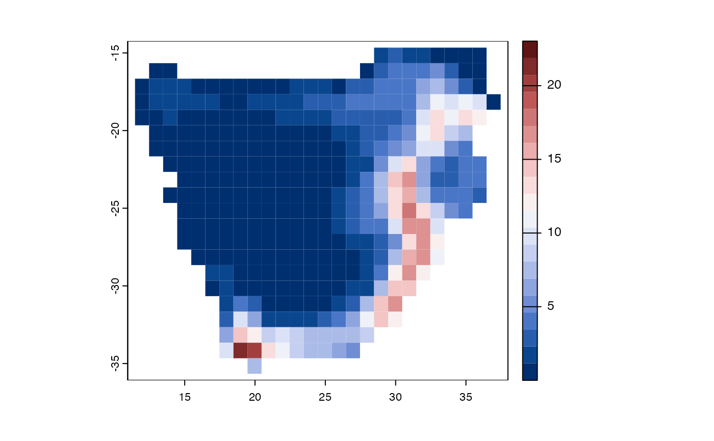

Figure 4. Geographic distributions of weighted endemism for woody plants of southern Africa.

Function PD – phylogenetic diversity

Phylogenetic diversity (PD) represents the length of evolutionary pathways that connects a given set of taxa on a rooted phylogenetic tree (Faith 1992). This metric is often characterised in units of time (millions of years, for dated phylogenies). We will map PD for plants of southern Africa.

data(africa)
comm <- africa$comm
tree <- africa$phylo
poly <- vect(system.file("ex/sa.json", package = "phyloregion"))

mypd <- PD(comm, tree)
head(mypd)

##    v3635    v3636    v3637    v3638    v3639    v3640 
## 4226.216 5372.009 4377.735 3783.992 3260.111 1032.685

M <- merge(poly, data.frame(grids=names(mypd), pd=mypd), by="grids")
M <- M[!is.na(M$pd),]
head(M)

##   grids       pd
## 1 v3635 4226.216
## 2 v3636 5372.009
## 3 v3637 4377.735
## 4 v3638 3783.992
## 5 v3639 3260.111
## 6 v3640 1032.685

par(mar=rep(0,4))
plot(M, "pd", border=NA, type="continuous",
            col = hcl.colors(20, "Blue-Red 3"))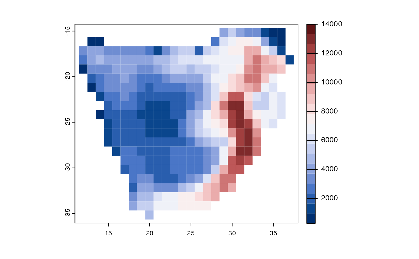

Figure 5. Geographic distributions of phylogenetic diversity for woody plants of southern Africa.

Function phylo_endemism – phylogenetic endemism

Phylogenetic endemism is not influenced by variations in taxonomic opinion because it measures endemism based on the relatedness of species before weighting it by their range sizes(Rosauer et al. 2009),(Barnabas H. Daru et al. 2020).

library(terra)
data(africa)
comm <- africa$comm
tree <- africa$phylo
poly <- vect(system.file("ex/sa.json", package = "phyloregion"))

pe <- phylo_endemism(comm, tree)
head(pe)

##     v3635     v3636     v3637     v3638     v3639     v3640 
## 32.536530 45.262625 35.004944 27.603721 23.183947  6.439589

mx <- merge(poly, data.frame(grids=names(pe), pe=pe), by="grids")
mx <- mx[!is.na(mx$pe),]
head(mx)

##   grids        pe
## 1 v3635 32.536530
## 2 v3636 45.262625
## 3 v3637 35.004944
## 4 v3638 27.603721
## 5 v3639 23.183947
## 6 v3640  6.439589

par(mar=rep(0,4))
plot(mx, "pe", border=NA, type="continuous",
            col = hcl.colors(n=20, palette = "Blue-Red 3", rev=FALSE))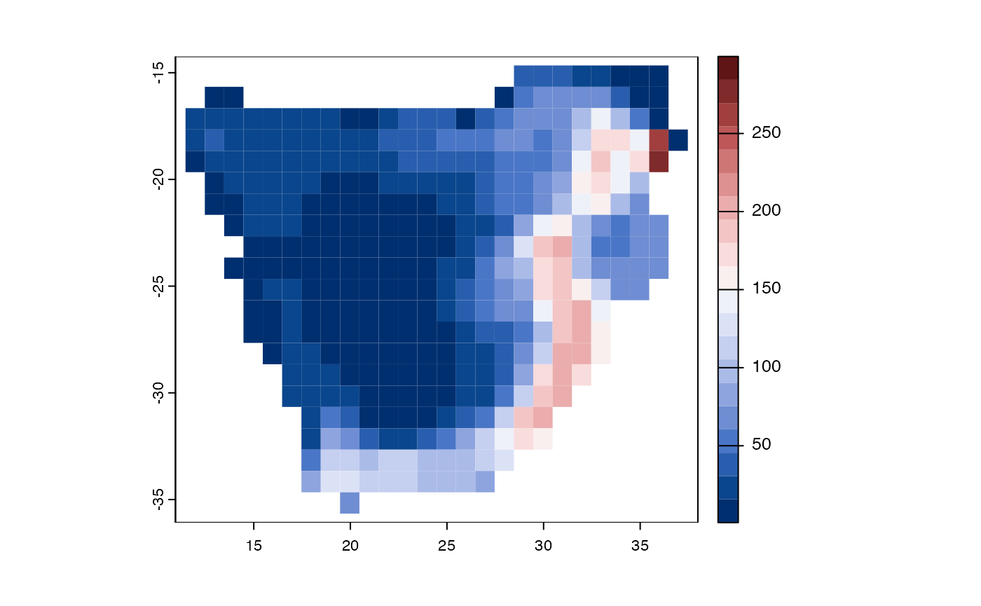

Figure 6. Geographic distributions of phylogenetic endemism for woody plants of southern Africa.

Function EDGE – Evolutionary Distinctiveness and Global Endangerment

This function calculates EDGE by combining evolutionary distinctiveness (ED; i.e., phylogenetic isolation of a species) with global endangerment (GE) status as defined by the International Union for Conservation of Nature (IUCN).

data(africa)
comm <- africa$comm
threat <- africa$IUCN
tree <- africa$phylo
poly <- vect(system.file("ex/sa.json", package = "phyloregion"))

x <- EDGE(threat, tree, Redlist = "IUCN", species="Species")
head(x)

##        Abutilon_angulatum_OM1934    Abutilon_sonneratianum_LTM034 
##                         2.903551                         2.903551 
## Acalypha_glabrata_glabrata_OM441  Acalypha_glabrata_pilosa_OM1979 
##                         2.480505                         2.480505 
##       Acalypha_sonderiana_OM2163  Acokanthera_oblongifolia_OM2240 
##                         2.914481                         2.211561

y <- map_trait(comm, x, FUN = sd, pol=poly)

par(mar=rep(0,4))
plot(y, "traits", border=NA, type="continuous",
            col = hcl.colors(n=20, palette = "Blue-Red 3", rev=FALSE))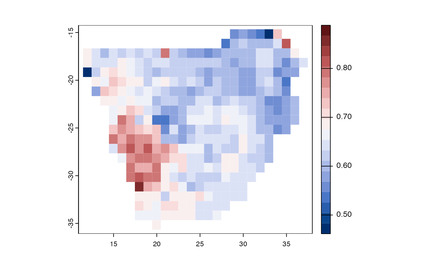

Figure 7. Geographic distributions of evolutionary distinctiveness and global endangerment for woody plants of southern Africa.

Analysis of beta diversity (phylogenetic and non-phylogenetic)

The three commonly used methods for quantifying -diversity, the variation in species composition among sites, – Simpson, Sorenson and Jaccard(Laffan et al. 2016). The phyloregion’s functions beta_diss and phylobeta compute efficiently pairwise dissimilarities matrices for large sparse community matrices and phylogenetic trees for taxonomic and phylogenetic turnover, respectively. The results are stored as distance objects for subsequent analyses.

---

Phylogenetic beta diversity

phyloregion offers a fast means of computing phylogenetic beta diversity, the turnover of branch lengths among sites, making use of and improving on the infrastructure provided by the betapart package(Baselga and Orme 2012) allowing a sparse community matrix as input.

data(africa)
p <- vect(system.file("ex/sa.json", package = "phyloregion"))
sparse_comm <- africa$comm

tree <- africa$phylo
tree <- keep.tip(tree, intersect(tree$tip.label, colnames(sparse_comm)))
pb <- phylobeta(sparse_comm, tree)

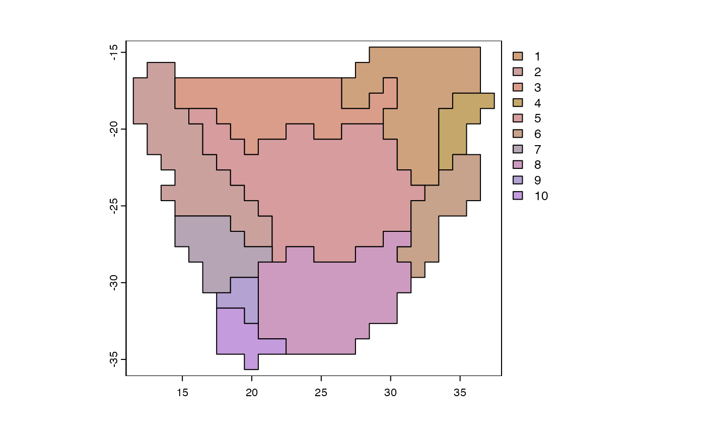
y <- phyloregion(pb[[1]], pol=p)

plot_NMDS(y, cex=3)

## Warning in mixcolor(seq(0, 199)/199, polarLUV(70, 50, 30), polarLUV(70, :
## convex combination of colors in polar coordinates (polarLUV) may not be
## appropriate

## Warning in mixcolor(seq(0, 199)/199, polarLUV(70, 50, 300), polarLUV(70, :
## convex combination of colors in polar coordinates (polarLUV) may not be
## appropriate

text_NMDS(y)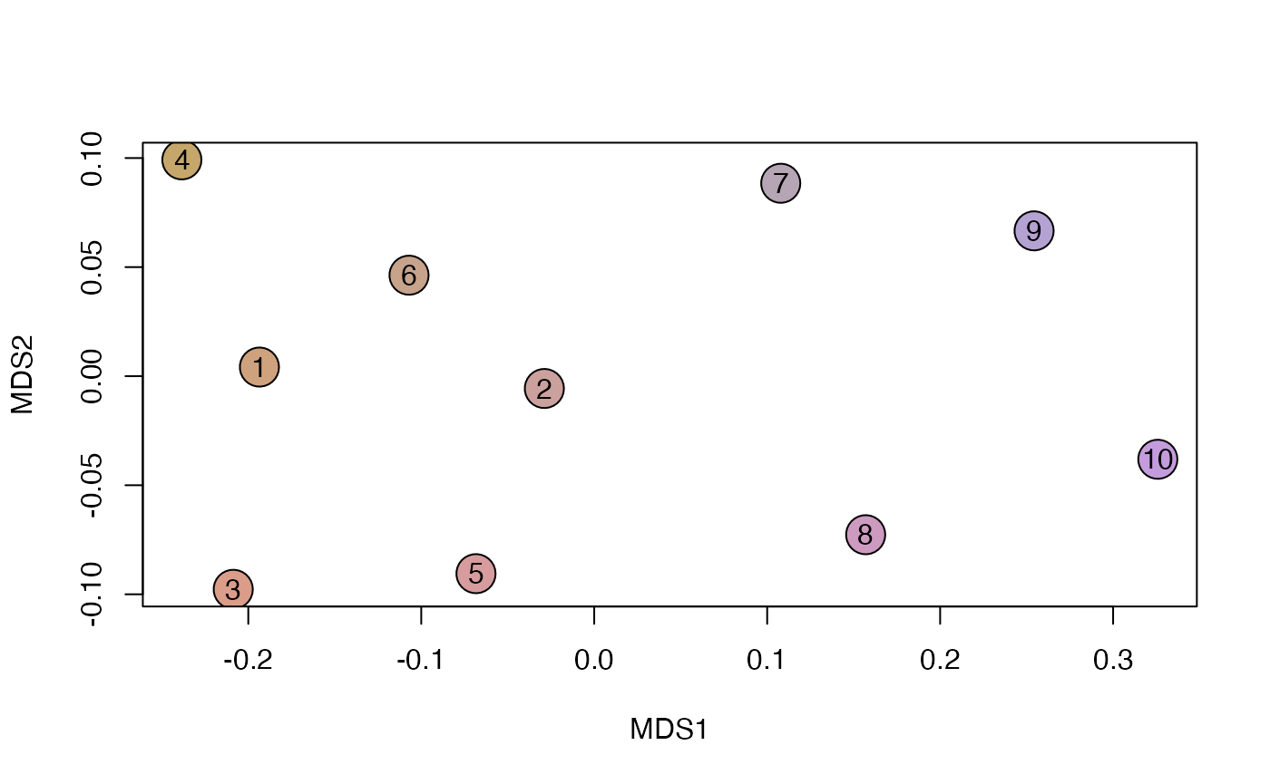

par(mar=rep(0,4))
plot(y, palette="NMDS")

Session Information

sessionInfo()

## R version 4.3.2 (2023-10-31)
## Platform: aarch64-apple-darwin20 (64-bit)
## Running under: macOS Sonoma 14.3
## 
## Matrix products: default
## BLAS:   /Library/Frameworks/R.framework/Versions/4.3-arm64/Resources/lib/libRblas.0.dylib 
## LAPACK: /Library/Frameworks/R.framework/Versions/4.3-arm64/Resources/lib/libRlapack.dylib;  LAPACK version 3.11.0
## 
## locale:
## [1] en_US.UTF-8/en_US.UTF-8/en_US.UTF-8/C/en_US.UTF-8/en_US.UTF-8
## 
## time zone: America/Los_Angeles
## tzcode source: internal
## 
## attached base packages:
## [1] stats     graphics  grDevices utils     datasets  methods   base     
## 
## other attached packages:
## [1] terra_1.7-55      Matrix_1.6-1.1    ape_5.7-1         phyloregion_1.0.9
## 
## loaded via a namespace (and not attached):
##  [1] fastmatch_1.1-4    xfun_0.41          bslib_0.6.1        clustMixType_0.3-9
##  [5] lattice_0.21-9     quadprog_1.5-8     vctrs_0.6.5        tools_4.3.2       
##  [9] doSNOW_1.0.20      generics_0.1.3     parallel_4.3.2     tibble_3.2.1      
## [13] fansi_1.0.6        cluster_2.1.4      highr_0.10         pkgconfig_2.0.3   
## [17] RColorBrewer_1.1-3 desc_1.4.2         lifecycle_1.0.4    compiler_4.3.2    
## [21] stringr_1.5.1      predicts_0.1-11    textshaping_0.3.7  minpack.lm_1.2-4  
## [25] smoothr_1.0.1      codetools_0.2-19   permute_0.9-7      htmltools_0.5.7   
## [29] snow_0.4-4         sass_0.4.8         yaml_2.3.7         pillar_1.9.0      
## [33] pkgdown_2.0.7      jquerylib_0.1.4    MASS_7.3-60        cachem_1.0.8      
## [37] vegan_2.6-4        iterators_1.0.14   abind_1.4-5        foreach_1.5.2     
## [41] maptpx_1.9-7       nlme_3.1-163       picante_1.8.2      phangorn_2.11.1   
## [45] digest_0.6.33      stringi_1.8.2      slam_0.1-50        purrr_1.0.2       
## [49] splines_4.3.2      magic_1.6-1        rprojroot_2.0.4    fastmap_1.1.1     
## [53] grid_4.3.2         colorspace_2.1-0   cli_3.6.1          magrittr_2.0.3    
## [57] utf8_1.2.4         rmarkdown_2.25     igraph_1.5.1       ragg_1.2.6        
## [61] memoise_2.0.1      evaluate_0.23      knitr_1.45         rcdd_1.5-2        
## [65] geometry_0.4.7     mgcv_1.9-0         itertools_0.1-3    rlang_1.1.2       
## [69] Rcpp_1.0.11        glue_1.6.2         betapart_1.6       rstudioapi_0.15.0 
## [73] jsonlite_1.8.8     R6_2.5.1           systemfonts_1.0.5  fs_1.6.3

REFERENCES

Baselga, Andrés, and C David L Orme. 2012. “Betapart: An r Package for the Study of Beta Diversity.” Methods in Ecology and Evolution 3 (5): 808–12.

Bates, Douglas, and Martin Maechler. 2019. Matrix: Sparse and Dense Matrix Classes and Methods. https://CRAN.R-project.org/package=Matrix.

Crisp, MICHAEL D, Shawn Laffan, H Peter Linder, and ANNA Monro. 2001. “Endemism in the Australian Flora.” Journal of Biogeography 28 (2): 183–98.

Daru, Barnabas H., Michelle van der Bank, and T. Jonathan Davies. 2015. “Spatial Incongruence Among Hotspots and Complementary Areas of Tree Diversity in Southern Africa.” Diversity and Distributions 21 (7): 769–80. https://doi.org/10.1111/ddi.12290.

Daru, Barnabas H, Tammy L Elliott, Daniel S Park, and T Jonathan Davies. 2017. “Understanding the Processes Underpinning Patterns of Phylogenetic Regionalization.” Trends in Ecology & Evolution 32 (11): 845–60.

Daru, Barnabas H., Harith Farooq, Alexandre Antonelli, and Søren Faurby. 2020. “Endemism Patterns Are Scale Dependent.” Nature Communications 11 (1): 2115. https://doi.org/10.1038/s41467-020-15921-6.

Daru, Barnabas H., Piyal Karunarathne, and Klaus Schliep. 2020. “Phyloregion: R Package for Biogeographic Regionalization and Macroecology.” bioRxiv. https://doi.org/10.1101/2020.02.12.945691.

Duff, I. S. 1977. “A Survey of Sparse Matrix Research.” Proceedings of the IEEE 65 (4): 500–535. https://doi.org/10.1109/PROC.1977.10514.

Faith, Daniel P. 1992. “Conservation Evaluation and Phylogenetic Diversity.” Biological Conservation 61 (1): 1–10. https://doi.org/10.1016/0006-3207(92)91201-3.

Kaschner, K, JS Ready, E Agbayani, J Rius, K Kesner-Reyes, PD Eastwood, AB South, et al. 2008. “AquaMaps: Predicted Range Maps for Aquatic Species.” World Wide Web Electronic Publication, Wwwaquamapsorg, Version 10: 2008.

Kembel, S. W., P. D. Cowan, M. R. Helmus, W. K. Cornwell, H. Morlon, D. D. Ackerly, S. P. Blomberg, and C. O. Webb. 2010. “Picante: R Tools for Integrating Phylogenies and Ecology.” Bioinformatics 26: 1463–64.

Laffan, Shawn W, and Michael D Crisp. 2003. “Assessing Endemism at Multiple Spatial Scales, with an Example from the Australian Vascular Flora.” Journal of Biogeography 30 (4): 511–20.

Laffan, Shawn W, Dan F Rosauer, Giovanni Di Virgilio, Joseph T Miller, Carlos E González-Orozco, Nunzio Knerr, Andrew H Thornhill, and Brent D Mishler. 2016. “Range-Weighted Metrics of Species and Phylogenetic Turnover Can Better Resolve Biogeographic Transition Zones.” Methods in Ecology and Evolution 7 (5): 580–88.

Oksanen, Jari, F. Guillaume Blanchet, Michael Friendly, Roeland Kindt, Pierre Legendre, Dan McGlinn, Peter R. Minchin, et al. 2019. Vegan: Community Ecology Package. https://CRAN.R-project.org/package=vegan.

Paradis, E., and K. Schliep. 2018. “Ape 5.0: An Environment for Modern Phylogenetics and Evolutionary Analyses in R.” Bioinformatics 35: 526–28.

Rosauer, Dan, Shawn W. Laffan, Michael D. Crisp, Stephen C. Donnellan, and Lyn G. Cook. 2009. “Phylogenetic Endemism: A New Approach for Identifying Geographical Concentrations of Evolutionary History.” Molecular Ecology 18 (19): 4061–72. https://doi.org/10.1111/j.1365-294X.2009.04311.x.

Ter Braak, Cajo J. F., and I.Colin Prentice. 2004. “A Theory of Gradient Analysis.” In Advances in Ecological Research: Classic Papers, 34:235–82. Advances in Ecological Research. Academic Press. https://doi.org/10.1016/S0065-2504(03)34003-6.